Explanation of Relative Death Toll (with Pictures)
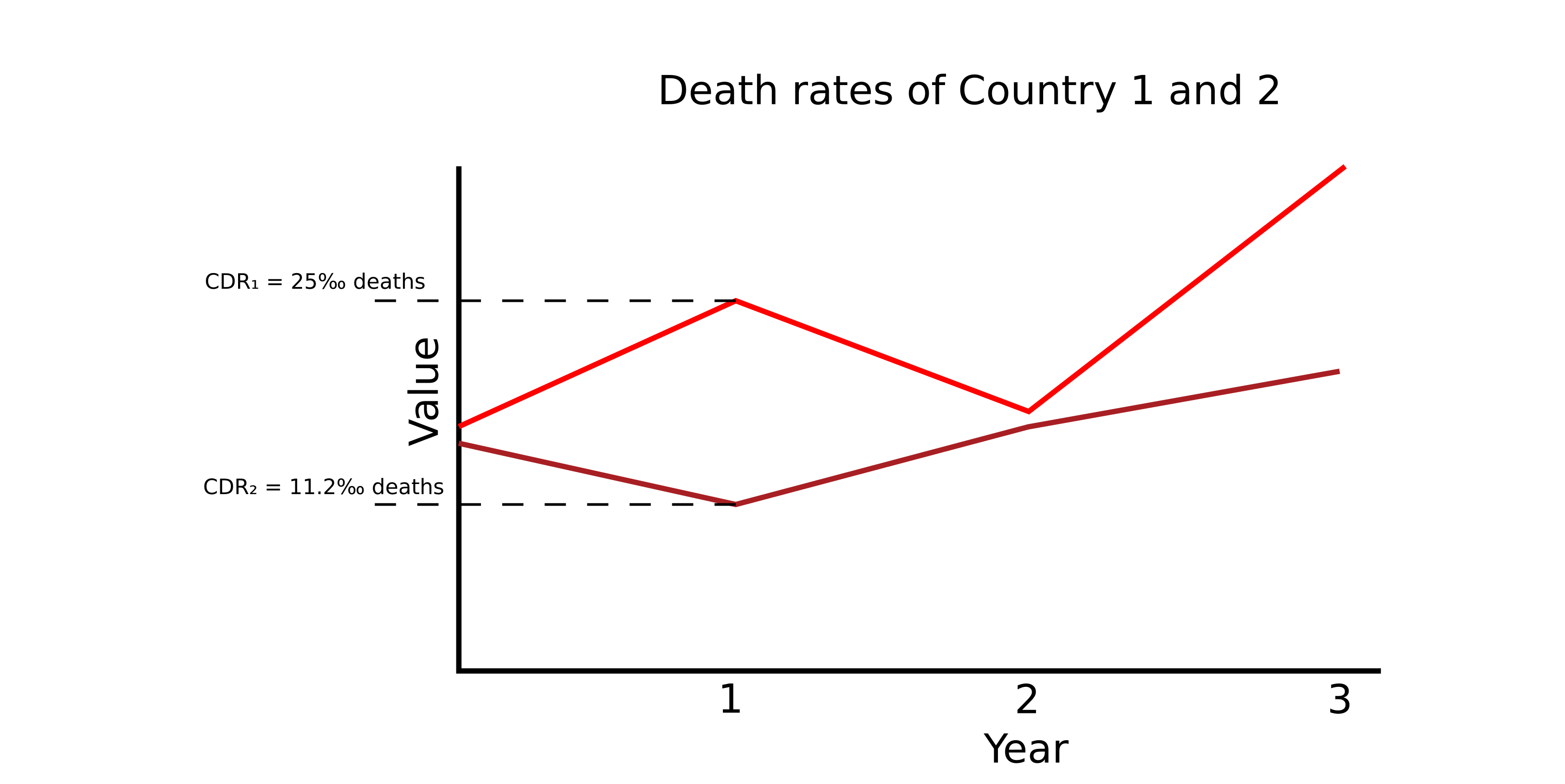
Figurex 1
Slides:(1) suppose over several years, the red and dark red lines correspond to the crude death rates (CDRs) per thousand people (‰) in two different countries (call them CDR₁ and CDR₂ respectively). (2) Suppose over those same years, the population for country 1 looks like this (call this population₁). (3) The total deaths in country 1 can be computed as CDR₁‰ × (population₁/1000); for example, for year 1, CDR₁ = 25‰, and population₁ = 40,000,000 ("40m"); so total deaths = 25*(40,000,000/1000) = 1,000,000 ("1 million"). This is shown on the bar graph as purple segments, although this is just for scale (and not to imply the population falls by that much per year, because it also gains a certain amount from births). (4) Let’s zoom in, and plot those total deaths per year for country 1. (5) If we take CDR₂ as our baseline, then we can compute the excess deaths based on the difference of the two CDRs (ΔCDR = CDR₁ - CDR₂, where "Δ" typically denotes "difference" or "change"). So, for example, in year 1, ΔCDR = 13.8‰, and CDR₁ = 25‰. So then "excess deaths" account for 13.8/25 = 55.2% of total deaths for country 1. The difference ΔCDR is much smaller for year 2, so then the excess deaths in that year are much smaller. (6) Over the period of interest, take the sum of these excess deaths for the total or "cumulative" excess deaths over that time interval.
Note: this graphic shows how to compute relative death toll between two CDR’s that change over time. If you are computing against a "simple" baseline (ie a value that remains unchanged over time), it would be like the above, except the dark red line stays at the same CDR value (ie is "flat") over the whole time.
Death is a part of life - but different factors make death more likely. For example, if country 1 has a much older population than country 2, that could explain the higher CDR. However, if two countries have a similar age structure, other factors must explain the difference in death rate, such as food shortage, disease, and so on.
If we think two countries are comparable, we would expect their death rates to stay similar. If they begin to diverge (ie ΔCDR ≠ 0), that indicates that something serious has happened in one of the countries - perhaps a more humane social policy, or perhaps an acute crisis. Either way, we can estimate how many people died in one country, due to this divergence in death rate.
Note this is the same method used to calculate excess death tolls in general. For example, during the Sars-CoV19 pandemic, we frequently heard about this, except the baseline used is a death rate from prior years in the same country.
Table India-I - Historical Populations of India; pre-1881 are averages of estimates (from Table India-III, India-VI; * at this point, populations are presented for what-will-become the Republic of India. Numbers in parentheses show the population in the British Raj. Also note in the 1830s, Burma (today: Myanmar) was separated from the British Raj.
Year
Population (1e6)
c. 1595
121.6 ± 16.8
c. 1650
90.0 ± 10.0
c. 1750
160.0 ± 34.9
c. 1800
176.9 ± 23.3
c. 1850
213.3 ± 21.4
1871
255.2/245.8 ± 13.3
1881
257.4
1891
282.1
1901
285.3
1911
303.0
1921
251.2(305.7)*
1931
278.9(338.2)*
1941
318.5(389.0)*
1951
361.0
Table India-II. From Table India-VI, India-VII. Note these are rough approximations. 1850-1871 is an average of the two regimes. Notice the Growth Rate is now per thousand (‰), not percent (%); data marked by * (in 1881) is obtained by using the CBR for the following period (1891), and computing CDR from that and the contemporary growth rate.
Interval
Growth Rate (‰ (per hundred))
Death Rate (‰, per thousand)
CBR regime/rate (‰, per thousand)
1650-1750
6.0‰ ± 2.5‰
36.5‰ ± 4.8‰
42.5‰ ± 4.1‰
1750-1800
1.7‰ ± 5.0‰
40.8‰ ± 6.5‰
42.5‰ ± 4.1‰
1800-1850
5.2‰ ± 2.7‰
37.3‰ ± 4.9‰
42.5‰ ± 4.1‰
1850-1871
4.0‰ ± 2.5‰
41.0‰ ± 4.9‰
45.0‰ ± 4.6‰
1871-1901
4.1‰ ± 0.97‰
43.4‰ ± 4.4‰
47.5‰ ± 4.3‰
1871-1881
0.09%
45.5‰*
46.4‰*
1881-1891
0.92%
37.4‰
46.4‰
1891-1901
0.11%
44.6‰
45.7‰
1901-1911
0.60%
39.9‰
45.9‰
1911-1921
0.09%
44.2‰
45.1‰
1921-1931
0.11%
34.9‰
45.4‰
1931-1941
0.13%
33.2‰
46.5‰
1941-1951
0.13%
32.4‰
44.9‰
For India? This is difficult to answer. Before the regular British censuses (a staggered one around 1871, and a standardized census every decade 1881 and beyond), the data is difficult. There are two pieces of information inferences of CDR are made from: population growth rate and fertility. A variety of population estimates are provided by Dyson (2018) for several points in Indian history, from which he estimates the intervening growth rates (GR) - we will re-compute these growth rates to determine error bounds as well. Second, fertility rates are roughly known, although as we’ll see, there is some subtlety in how this may have changed over time, and thus, in conjunction with changing age structure, how CBR changed over time. Assuming then negligible in or out migration, we can estimate CDR as GR - CBR. We will review the variable results possible from different interpretations to get a picture of mortality trends over time. Based on the growth rates supplied by Dyson’s data, and following work suggesting increasing CBR over time, I lean towards a CDR regime in the pre-colonial normal times - our putative baseline - around 36.5‰ ± 4.8‰.
Table India-III. Population estimates, Dyson (2018) Table 4.1 and Table 5.1; those with † from Visaria and Visaria, Table 5.1; * from Sumit Guha (2001a)
Author
c. 1595 Estimate
c. 1650 Estimate
c. 1750 Estimate
c. 1800 Estimate
c. 1850 Estimate
Moreland
100m
-
-
-
-
Davis
125m
-
-
-
-
Datta
110m
-
-
-
-
Das Gupta
135m
-
-
-
-
Habib
142m
-
-
-
-
Moosvi
145m
-
-
-
-
Sumit Guha
116m
-
-
161m*
-
Swaroop and Lal
-
-
102m
139m
183
Shirras†
-
80
130
190
Carr-Saunders†
-
100
-
-
205
Sen Gupta†
-
-
-
179m
223
Willcox
100†/-†
100m†/80m†
144†/130m
-†/157m
205/190
Bhattacharya
-
-
190m
207m
247
Clark
-
-
200m
190m
-
Durand
-
-
160-214m
160-214m
215/233/242
McEvedy and Jones
-
-
170m
185m
-
From 1750 to the early 19th century, the Indian subcontinent was submerged in a broad crisis of war, famine, and disease, which some scholars argued lead to a population decline (although not all agree here). Company rule after this was an improvement, although the Company was part of the problem in that chaotic era (yet not solely responsible). As Dyson (2018) notes, population growth rates were likely around 0.2-0.4%, which for the 19th century (ie 2-4 new persons per thousand, per year), and Indian history of the past few thousand years, was significant - from 640 to 1595 CE, the growth rate was probably 0.1% at most (1 new person per thousand, per year). Further, from 1750 to 1800, he guestimates the growth rate at 0.1%. He argues thus that, "birth rates being uncontrolled", this must have been a result of a slightly lower mortality rate. He doesn’t quite praise Company rule, but concludes this was probably a result of Pax Britannica - which is reasonable, given this data.
(Dyson doesn’t give errors; these can be computed for his method however; see table; for 640, an error of 10m was used for the given population estimate (58m); it’s unclear how to compute this for that year, but Dyson clearly argues there is substantial margin of error. For other years, the population is the average of the given set of population estimates (per Dyson), and the error is the standard deviation. When no data set is given, (1650, 1850, 1871, and 1901), the data set is from Visaria and Visaria (YEAR), which Dyson relies on heavily. How Dyson calculated the average for 1750 and 1800 is a little unclear to me, so I present results for Dyson’s number (using my error), indicated with an asterisk (*). For my calculations, I use the average from Visaria and Visaria for 1850 and 1871 (Dyson uses the mode, and that number is used for (*) entries). Growth rate (and its error) between two years x₁ and x₂ is determined by fitting an exponential curve A×exp(-rx), where x is year (years shifted so x₁ = 0), A is the initial population, and r is the growth rate.)
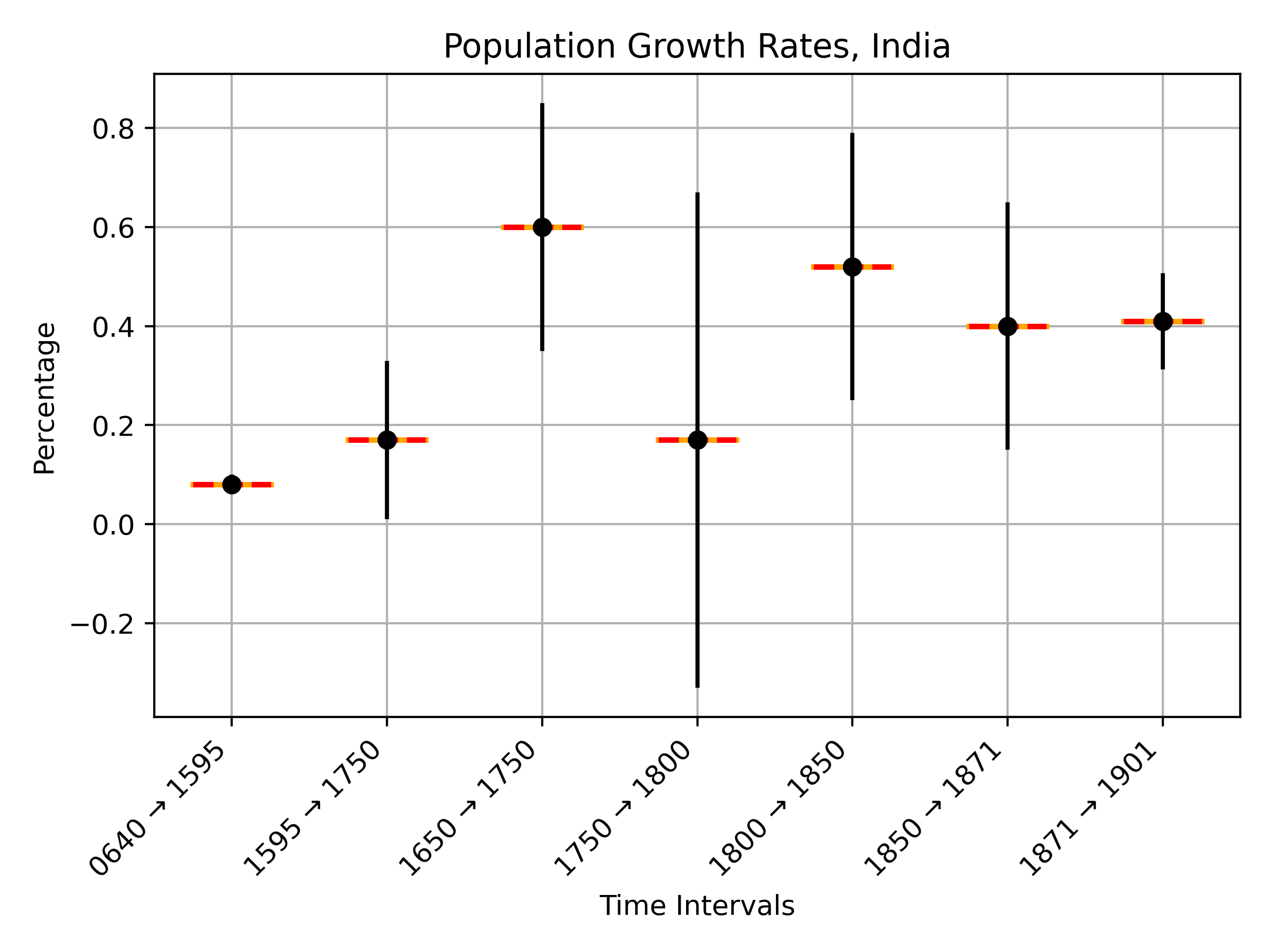
Table India-IV.
Interval
Growth Rate
640-1595
0.08% ± 0.02%
1595-1750
0.17% ± 0.16%
1650-1750
0.6% ± 0.25%
1750-1800
0.17% ± 0.5%
1800-1850
0.52% ± 0.27%
1850-1871
0.4% ± 0.25%
1871-1901
0.41% ± 0.097%
1800-1871*
0.44% ± 0.093%
1800-1871
0.5% ± 0.18%
However, there a few issues here. First, he is comparing a period of fairly solid peace to an interval of nearly 1000 years (containing both periods of prosperity and despair), and to a 50 year period of historic strife. Setting aside the former, the latter clearly should underperform for the reasons he lists. It also begs the question - what was growth like during the [more geographically limited] "Pax Mughalica"? Using the population estimates for 1595 to 1750 (although not a perfect overlap) given by Dyson, we get 0.17% ± 0.16%. This is still notably larger than 0.1%. Further, using the 1650 estimates from Visaria and Visaria until 1750, we get 0.6 ± 0.25%. What this suggests is over periods of relative stability, growth rates in India could be substantial, slightly larger than in the 19th century, although difficult to statistically distinguish.
The second problem has to do with birth rates; Dyson guestimates a CBR of 46‰. In fact, Dyson reports that Indian birth rates were quite controlled - on average, 5-6 per woman over their fertile ages (that is, if an Indian woman survived through menopause, on average they would have around 5-6 children), leaning towards 6 (which seems to be the 5.8 from Sellier (1989), rooted in ancient Pakistan, but seems to be consistent with known fertility rates over time; this value itself has an error of 0.74). It’s worth remarking that in China, with a similar fertility level, the estimated historical CBR ranged 37-42 (Maddison CITE), although this could be slightly lower due to a different age composition. Next what age range for fertility? Per female age structure from 1901 (Mukherjee 1976), that’s about 46% if ranging from 15-45, and 49% if from 15-49 (child marriage, and teenage pregnancy, was typical). Taking the average of the rough CBR from these two ranges, and accounting for a slight imbalance towards men (say, women were 49.5% of the population), we get CBR’s of 44 and 41‰ FORMULA
The formula used here is CBR = (fertility/age-span)*(total-number-of-child-bearing-women per 1000 people); so using the 15-45 age-span (covering 46% of the female population), we get CBR = (5.8/30)*(0.46*0.495*1000) = 44.022 , respectively - the "average" of these being 42.5‰ ± 4.1‰ FORMULA
This is a pretty rough error. Because the underlying origin of the two values, 41‰ and 44‰, are obtained in different ways, we have two sources of error: the error of the mean of the two data points themselves: (stddev/√(2) = 2.121320344/√(2) = 1.5) and the error of the mean resulting from the propagation of the error of the data points. This comes from the 0.74 fertility error: thus, for 15-45, we have (0.74/30)*(0.46*0.495*1000) = 5.6166 (ie CBR = 41 ± 5.6) and for 15-49 we have (0.74/35)*(0.49*0.495*1000) = 5.1282 (ie CBR = 44 ± 5.1). Thus, σ_{μ}² = σ₁²(1/n²) + σ₂²(1/n²) = 5.6166*(1/4) + 5.1282*(1/4) = 14.4611577, and thus σ_{μ}² = 3.802782889. So then the overall error, as a rough value, is taken as σ = √(3.802782889² + 1.5²) = 4.087928290, which we can round to 4.1. , quite a bit lower than Dyson’s 46‰ (although it’s within the first confidence interval, so not statistically alarming). Altogether, our error is growing large - about 7-8‰ [???]. Since, assuming in or out migration didn’t affect population much (as Dyson suggests is approximately true), CDR = CBR - R, we must include our R errors, thus our CDR errors range from 7 to 9.
Table India-V.
Interval
Growth Rate
Death Rate (CBR: 42.5‰ ± 4.1‰)
Death Rate (CBR: 47.5‰ ± 4.3‰)
640-1595
0.08% ± 0.02%
41.7‰ ± 4.1‰
46.7‰ ± 4.3‰
1595-1750
0.17% ± 0.16%
40.8‰ ± 4.4‰
45.8‰ ± 4.6‰
1650-1750
0.6% ± 0.25%
36.5‰ ± 4.8‰
41.5‰ ± 5.0‰
1750-1800
0.17% ± 0.5%
40.8‰ ± 6.5‰
45.8‰ ± 6.6‰
1800-1850
0.52% ± 0.27%
37.3‰ ± 4.9‰
42.3‰ ± 5.1‰
1850-1871
0.4% ± 0.25%
38.5‰ ± 4.8‰
43.5‰ ± 5.0‰
1871-1901
0.41% ± 0.097%
38.4‰ ± 4.2‰
43.4‰ ± 4.4‰
1800-1871*
0.44% ± 0.093%
38.1‰ ± 4.2‰
43.1‰ ± 4.4‰
1800-1871
0.5% ± 0.18%
37.5‰ ± 4.5‰
42.5‰ ± 4.7‰
Table India-VI. British Raj/Republic of India inferred vital metrics (1871-1921: Dyson 2018 Table 7.1; 1921-1971: Dyson 2018 Table 8.1); note for some 1921 data, and for 1931 and beyond, the metrics are for the current territory of the Republic of India; otherwise, the data is for territory of the British Raj (where both data present, the Raj data is in parentheses); data marked by * (in 1881) is obtained by using the CBR for the following period (1891), and computing CDR from that and the contemporary growth rate.
Year
Population (1e6)
Growth Rate (%)
Sex Ratio (m:f)
Life Expectancy M/F
CDR(‰)
CBR (‰)
fertility/woman
female marriage age
1871
255.2
-
1.059
-
-
-
-
-
1881
257.4
0.09
1.040
-
45.5*
46.4*
-
-
1891
282.1
0.92
1.042
26.3/27.2
37.4
46.4
5.81
-
1901
285.3
0.11
1.037
22.2/23.4
44.6
45.7
5.78
-
1911
303.0
0.60
1.047
25.3/25.5
39.9
45.9
5.77
-
1921
251.2(305.7)
0.09
1.047(1.056)
21.8/22.0
44.2
45.1
5.75
12.7
1931
278.9(338.2)
0.11
1.053
29.6/30.1
34.9
45.4
5.86
12.7
1941
318.5(389.0)
0.13
1.058
29.5/29.6
33.2
46.5
5.98
14.2
1951
361.0
0.13
1.057
31.0/31.8
32.4
44.9
5.96
15.6
1961
439.1
0.20
1.063
36.8/36.6
25.9
45.5
6.11
16.1
1971
548.2
0.22
1.075
44.0/43.0
21.3
43.5
6.50
17.1
The third problem is, despite writing about fertility control measures, his assertion that fertility was actually "uncontrolled", and thus variations in R must be a result of variations in CDR. In fact, Dyson co-authored a seminal paper on how fertility is socially determined; the more subordinated and isolated women are, the more children they are made to bear (Dyson 1983?) (ie fertilities at or above 7). Parthasarathi (2001) cites work from Sumit Guha (2001) indicating that fertility rates in 18th century and early 19th century India were probably lower than in the late 19th century and early 20th century, due to differing family structures, closer to a nuclear structure in the earlier era, with joint-household structures gaining more prominence in the latter period. Nuclear families typically have lower fertility levels than joint-households, the latter associated also with increasing disempowerment of wives (ie Dyson 1983).
EDIT INTO NARRATIVE: Thus, the lower fertility regime in Table India-V (under the column "Death Rate (CBR: 42.5‰ ± 4.1‰)") may be more representative of India up to (and including) the early 19th century (see the condensed Table India-VII). Note that these numbers are obtained from a fertility rate of 5.8 and 6.5 applied to the age structure of India in the turn of the 20th century. But the recorded fertility in the turn of the century was around 5.8; the lower CBR of earlier times would be due to a slightly lower fertility rate, and an older age structure (as suggested by Parthasarathi (2001), referring to patterns in late 19th century Berar observed by Dyson (1989)). This is a crude calculation however, and CBR values around 46 were obtained from more sophisticated life table calculations (ie Dyson (2018)) with a fertility of 5.8 (not 6.5), and the contemporary age distribution.
EDIT INTO NARRATIVE: using 36.5‰ as the baseline, we get about 59m excess deaths from 1881-1921. (hickesullivanRedo.py)
Table India-VII. Note these are rough approximations. 1850-1871 is an average of the two regimes. Notice the Growth Rate is now per thousand (‰), not percent (%)
Interval
Growth Rate (‰)
Death Rate
CBR regime
1650-1750
6.0‰ ± 2.5‰
36.5‰ ± 4.8‰
42.5‰ ± 4.1‰
1750-1800
1.7‰ ± 5.0‰
40.8‰ ± 6.5‰
42.5‰ ± 4.1‰
1800-1850
5.2‰ ± 2.7‰
37.3‰ ± 4.9‰
42.5‰ ± 4.1‰
1850-1871
4.0‰ ± 2.5‰
41.0‰ ± 4.9‰
45.0‰ ± 4.6‰
1871-1901
4.1‰ ± 0.97‰
43.4‰ ± 4.4‰
47.5‰ ± 4.3‰
EDIT INTO TEXT: These ambiguities are reflected in ambiguities in life expectancy. From 1871-1921, Dyson (2018) estimates this at 22-27 years (Ch. 7 section "Population Trends"), and from 1821-1871, at most 25 years (Ch. 6 Section "Demographic Characteristics"). In the Mughal era, Faruqi (2009) suggests life expectancy couldn’t have been more than 30 years, at least in the late 17th and early 18th centuries. Yet Parthasarathi (2005) argues that 18th century living standards were comparable to contemporary England. At very least, the picture drawn from Faruqi and Dyson suggests a decline in life expectancy, qualitatively consistent with the picture painted thus far of overall increasing CDR.
Using a fertility of 6.5, for example, yields CBR’s of 45.6-49.4, or 47.5 ± 4.3‰ FORMULA
The error of the mean of the two data points themselves: (stddev/√(2) = 2.687005769/√(2) = 1.9) and the error of the mean resulting from the propagation of the error of the data points. This comes from the 0.74 fertility error: thus, for 15-45, we have (0.74/30)*(0.46*0.495*1000) = 5.6166 (ie CBR = 49.4 ± 5.6) and for 15-49 we have (0.74/35)*(0.49*0.495*1000) = 5.1282 (ie CBR = 45.6 ± 5.1). Thus, σ_{μ}² = σ₁²(1/n²) + σ₂²(1/n²) = 5.6166*(1/4) + 5.1282*(1/4) = 14.4611577, and thus σ_{μ}² = 3.802782889. So then the overall error, as a rough value, is taken as σ = √(3.802782889² + 1.9²) = 4.251018431, which we can round to 4.3. (depending on the fertility window used) - a difference of about 5 from our prior CBR value. This could more than compensate for an increase in R from 0.1 → 0.2-0.4. Further, taking Pax Mughalica CBR as 42.5, and the associated growth rate R of 6‰, we get a CDR of 36.5±7.5.
Altogether then, what we see is that peacetime 19th century India faced growth which may have been slightly higher than normal, or may have been typical, and possibly not the highest to that point. Note that Dyson quotes the following:
the condition of the lower sectors of society in Bihar and eastern UP improved more...between the 1840s and 1870s than the literary evidence suggests [and that] despite the increasing population densities and the imbalanced rewards of the commercialization of the economy, these people experienced superior nutrition and health during their formative years. - Brennan et al. (1994), pg 289, 'The Heights of Economic Well-being of North Indians under British Rule'
Yet, with this look at the data, such an interpretation seems questionable. If birth rates were higher (that is, truly "uncontrolled" in the Malthusian sense (not socially uncontrolled, however)), then the same (or a similar) growth rate would be achieved as in Pax Mughalica, albeit with a higher CDR. It’s worth noting that Visaria and Visaria report birth rates of 38-41 in two central Indian districts in the early 19th century, although they assert the CBR was probably higher (pg 484). Further, for the late 19th century - when demographic data is more reliable, due to the post-1871 censuses - Visaria and Visaria record three of four demographers estimating CBR in the high 40s (themselves estimating 51.4 for 1891-1901) (pg 508). Note, this is consistent with Dyson’s CBR of 46 - the issue is that 46 is not necessarily representative of earlier CBRs.
Given the large error here, it’s difficult to draw a firm conclusion. There is little hard evidence on growth rate, death rate, or birth rate (other than that CBR is probably greater than 42 is a decent assumption for pre-modern Indian history, and that R is likely between 1% and 0.1%). Thus, while the data is plausibly consistent with Dyson’s argument that CDR declined from its historical average (and perhaps in some sub-intervals of the 19th century, it did; especially if we take CBR as the same for the Mughal and British period, which may also be plausible as a first guess), it’s also consistent with both birth and death rates increasing. This is consistent with the social argument that the 19th century saw a further subordination of women (particularly in northern India (Dyson 1983?)), and with the "literary evidence" that suggests the "condition of the lower sectors of society" deteriorated, and thus that death rates increased (ie from the putative Mughal average of 36.5, to the 19th century average of 42.3-43.5). This seems compelling to me, although one could statistically argue both CBR increased and CDR declined.
What is clear is that the agrarianate demographic regime remained in place during most of British colonial rule, and even in the 1940s, CDR remained in the 30s. This was a decline from the 1880-1920, although it was a strikingly high death rate. These facts alone damn the mythos that the British were a "progressive" force, as their impact on India’s vital rates is ambiguous at best - surely a "progressive" force should have made significant dents in a "feudal" demographic regime. This task would instead be tackled by the independent states of Pakistan, Bangladesh, and India.