There are many ways to measure, and compare, the well-being of a population. Today life expectancy is predominant, but one could also look at crude death and birth rates (CDR and CBR), which is the number of deaths per 1000 people in a population. So if there are 51,835 deaths in a country with a population of 893,831 over a year, then CDR = (51835/(893831/1000)) = 58‰, which is extremely high. For the population to maintain that year, then the CBR would have to be at least that value. While a useful metric for looking at mortality deviations, or a crude picture of the death and birth relationship, the utility of CDR/CBR becomes more fraught as age-structure changes. For example, if country 1 had a CDR of 20, and country 2 had a CDR of 10, it may appear that country 2 is much healthier. Yet if country 1 is also much older, interpreting the mortality discrepenacy is made harder, since old people tend to die easier than the younger. So how to compare these countries?
On the other hand, life expectancy is based on the probability of surviving from one age bracket to another (ie P(0 → 1), P(1 → 2), etc), which altogether can be used to estimate a life expectancy. This metric works no matter how many people are in any age bracket (MORE), and so today, as societies have many subtle variations in age structure, its more useful. Plus, "life expectancy" is much easier to apply to yourself: if I live in Japan, I can expect to live longer than if I’m American. One issue with this metric in older periods, however, is that infant mortality has been high until very recently. Thus, there were two times in life when you were peak likely to die: as an infant, and as you grew older. But taking averages over a "bimodal" distribution (as its technically called - ie two peaks) obscures this information, and suggests the average is at an improbable value. So medieval people, for example, didn’t live on average to 30. They either died an infant, or survived into their 40s to 60s. But these days, infant mortality is generally low, or at least not a significant peak relative to old people, and so life expectancy more meaningfully reflects an expected life time.
However, CDR and CBR are still very useful (and can be made more precise by looking at CDR and CBR in age brackets, a very similar reckoning as for life expectancy) - for example, during COVID, estimates of mortality were computed by calculating how many people were expected to die in a year, versus how many actually did.
Demography Basics
Demography is the study of populations and their dynamics. What is the age distribution of a population? The sex/gender distribution? The life expectancy? How does probability of death vary over age and sex/gender? How does fertility†
Note: Within demography, "fertility" is the actual number of children produced by a population (as a whole, over a given period of time, in a certain age-group, or any such population slice); "fecundity" refers to the maximum potential. However, in common usage (and other fields), "fertility" is often used in a similar way as "fecundity". For example, you might hear about fertile soil, referencing soil which has the potential to grow a lot of crops. This is a slightly different meaning than here. vary over age groups? What is the overall "crude" death and birth rate of a population? What is the overall growth rate of a population?
In much of the work here - looking at the health profile of different social relations - the main concern is the crude death rate (CDR), which is how many people die per thousand people in a year, written as X‰ (ie 35‰ = 35 deaths per 1000 people per year, or 35 deaths/1000 people/year). Often however, the literature gives a variety of other metrics. So it’s important to understand these.
Some metrics, such as CDR and crude birth rate (CBR), depend on the age distribution (AD) of a population (CDR and CBR, along with marriage statistics, are often referred to as "vital statistics"). While age-specific death rate (DR) and birth rate (BR) metrics are obtained, we can get a profile for population growth from the crude rates: assuming no (or negligible) immigration/emmigration, then the population growth rate per thousand persons (PGR) can be computed as:
PGR = CBR - CDR (Eqn. 1)
Yet, as mentioned, these are AD dependent statistics. For example, a hypothetical population that is 100% older than 70 years will likely have a higher CDR than a typical AD population (say, for the sake of numbers, 90‰ CDR vs 11‰ CDR), and will probably have a 0‰ CBR (vs say 14‰ CBR). It might therefore look like the old population lives under a very horrible social system, with a death rate 8x higher! But the fact that the AD is so different means we can’t be entirely sure if that’s the reason - or if its more just a result of our mortal coils.
These age-dependent metrics (ADM/ADMs) were once much more in fashion - back in the early 20th century, most of the world still lived in the high CDR/high CBR regime (HDHB-R), although the West had well begun its "demographic transition" to the low CDR/low CBR regime (LDLB-R) (why?
This is a fairly complex phenomena, but the demographic fact is: if a population has a high CDR, then a high CBR is required to avoid a negative PGR (see Eqn. 1). As nutrition, sanitation, and healthcare access grows, CDR declines, and CBR can decline as well. However, falling CDR doesn’t necessarily yield a falling CBR: in mid-20th century Latin America, for example, falling CDR was accompanied by a rising CBR! (CITE Albornoz).). Because these demographic regimes were fairly stable in the "Third World" (Global South), CDR and CBR gave fairly reliable demographic pictures over time.
Yet the age-dependency is a bit of a confounding factor here. So age-independent metrics grew in favor recently, most notably life expectancy [at birth] (LEAB). Such metrics are based on the survival rates of age cohorts, but not the AD of such cohorts. So if one country is much older than another (but there must be some people in all cohorts, else the survival rate in an age cohort is undefined), the LEAB is still comparable: if the LEAB of country A is 75, and the LEAB of country B is 82, then it is apparent that country B is overall "healthier".
Sen-Dreze Comparison (Method Explanation)
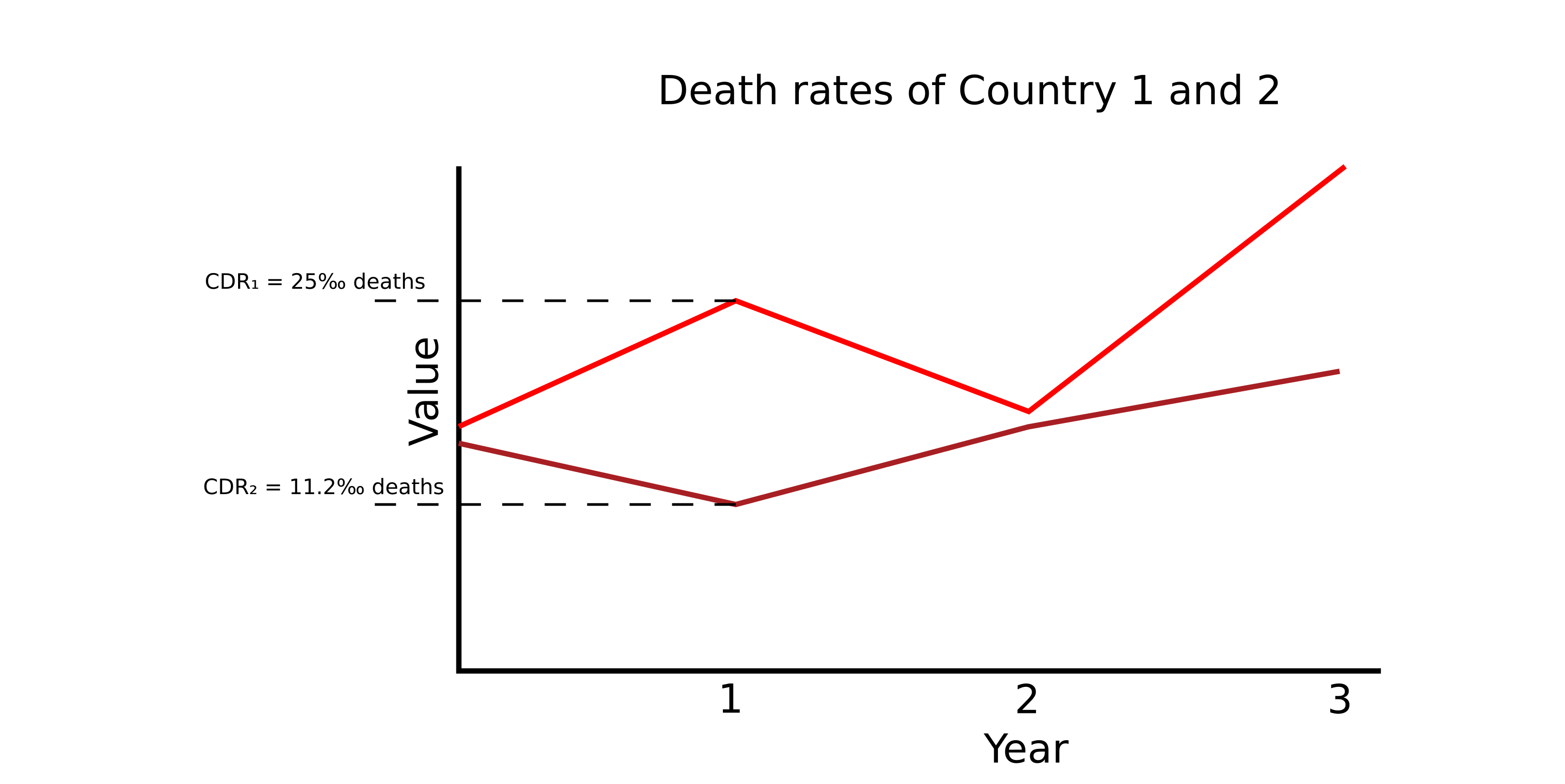
Figurex 1
Death is a part of life - but different factors make death more likely. For example, if country 1 has a much older population than country 2, that could explain the higher CDR. However, if two countries have a similar age structure, other factors must explain the difference in death rate, such as food shortage, disease, and so on.
If we think two countries are comparable, we would expect their death rates to stay similar. If they begin to diverge (ie ΔCDR ≠ 0), that indicates that something serious has happened in one of the countries - perhaps a more humane social policy, or perhaps an acute crisis. Either way, we can estimate how many people died in one country, due to this divergence in death rate.
Note this is the same method used to calculate excess death tolls in general. For example, during the Sars-CoV19 pandemic, we frequently heard about this, except the baseline used is a death rate from prior years in the same country.
Life Table Stuff
following cohort over time, record number of individuals alive at each birthday (age x), and number dying during following year (between x and x+1) - denoted q(x). Once all q(x) known, life table completely determined. "Cohort life tables" not used, but "period/current life table" - summarizing q(x) ∀ x in a short period (1 or 3 years), where q(x) is the death probability. (1).
The following are some of the standard actuarial functions:
mₓ [3] / m(x) [1] := mortality rate at age x [1] / "central death rate" [3] - estimated from data, sole input to life table. All are other quantities determined once m(x)’s specified. By construction:
m(x) = d(x)/L(x) [1,3 eqn 5]
mₓ = dₓ/nₓ (for stationary population) [3, eqn 3]
that is, number of deaths at age x, divided by number of person-years at risk at age x. Note m(x) and q(x) aren’t identical. For one year interval will be close, but m(x) always larger
Note that mₓ can exceed 1 [3]
Lₓ [3] / L(x) [1] := total number of person-years lived by the cohort [x,x+1) [1] / "average number living at age x during the year" [3] - sum of the years lived by the I(x+1) persons who survived the interval and d(x) persons who die during the interval. The former contribute 1 ea, latter on avg approx half year; so:
L(x) = I(x+1) + 0.5*d(x) [1]
L_x = ∫_0^1 l_{x+t}dt [3, eqn 4]
This works except for age 0 and oldest age, special calculations here.
d(x) := number of deaths in the interval [x,x+1) for people alive at age x, computed as:
d(x) = I(x) - I(x+1) [1]
d_x = l_x - l_{x+1} [3, eqn 1]
So if I(50) = 89867, I(51) = 89301, then d(50) = 89867-89301 = 566.
qₓ [3] /q(x) [1] := probability of dying at age x / age-specific risk of death [1] / probability of dying within 12 months [3] / "mortality rate" [3] - generally derive via
q(x) = 1 - exp[-m(x)]
assuming that the "instantaneous mortality rate" or "force of mortality" constant {μₓ} in the interval [x,x+1). By construction,
q(x) = d(x)/I(x) [1]
qₓ = dₓ/lₓ [3, eqn 2]
Note that qₓ can never exceed 1 [3]
μₓ - force of mortality / hazard rate [3] - obtained when we compute mₓ over shorter and shorter periods of time, calculus:
μₓ = -(1/lₓ)(dlₓ/dx) [3, eqn 6]
lₓ [3] / I(x) [1] := "survivorship function" [1] / number who survive to reach the exact age x[3] / "survival function" [3] - number of people alive at age x. ie I(50) = 89.867%. Computed recursively from m(x) values via
I(x+1) = I(x)*exp[-m(x)]
With I(0) arbitrary set to 100k. Example: I(2) = I(1)*exp[-m(1)] = 98961*exp[-0.00078] = 98883.
From [3 eqn 1+2] it follows that
1 - q_x = l_{x+1}/l_x [3 eqn 8]
T(x) := total number of person-years lived by the cohort from age x until all members of the cohort have died.
T(x) = Σ_{c=x}^{c=c_f}L(c)
Where c is "cohort" and c_f is "final cohort"
e(x) [1] / e̊ₓ [2] := the remaining life expectancy of persons alive at age x - computed as
e(x) = T(x)/I(x)
= ∑_{
Remarks
"The fundamental step in constructing a life table from population data is that of developing probabilities of death, qx, that accurately reflect the underlying pattern of mortality experienced by the population." (2)
Combine [3 eqn 8+9] and assume μ_x integral roughly close to μ_{x+(1/2)}, obtain
μ_{x+(1/2)} ≈ -ln(1 - q_x) [3 eqn 10]
q_x ≈ 1 - exp[-(μ_x + (1/2))] [3 eqn 11]
Combining [3 eqn 7+10+11]:
mₓ ≈ -ln(1 - qₓ) [3 eqn 12]
qₓ ≈ 1 - exp[-mₓ] [3 eqn 13]
By similar methods, can derive
μ_x ≈ -(1/2)ln[p_{x-1}p_x] [3 eqn 14]
Where pₓ = 1 - qₓ
Other Terms
stationary population - number of people who leave an age group x in a year (by reaching x+1 or dying) is exactly balanced by the number who reach the x age group; then nₓ is constant.